 Boring Log Viewer
Your first boring log
In this tutorial you'll draw a log for a 20 ft boring, starting with three layers and then adding samples, blow counts, lab results, groundwater and a header.
Step 0: Open the viewer
Go to uclageo.com/boring-log-viewer. The page has two halves:
- Left: a text box where the boring log data goes.
- Right: the drawn log, which updates as you type, with buttons to download it.
Click Clear to empty the text box. (To see a finished example first, choose one from Load example….)
The web page draws the log inside your browser. The data you type is not sent anywhere, and it is kept in your browser so it's still there if you reload the page.
Step 1: The layers
Copy this into the text box:
step1-layers.jsonDownload{
"schema_version": "1.0",
"units": { "length": "ft" },
"metadata": { "boring_name": "B-1" },
"layers": [
{ "top": 0, "bottom": 4, "description": "Brown, loose, moist, silty SAND (fill)" },
{ "top": 4, "bottom": 12, "description": "Gray, medium dense, wet, poorly graded SAND with silt" },
{ "top": 12, "bottom": 20, "description": "Gray, soft, wet, lean CLAY" }
]
}Here's what each part means:
"schema_version": "1.0"says which version of the format the file follows. It's optional: without it, the latest version (1.0) is assumed. Including it keeps the file readable if the format changes in the future."units": { "length": "ft" }says the depths are in feet. Leaveunitsout to use metres."metadata": { "boring_name": "B-1" }gives the log its title."layers"is the list of strata, from the top down. Each layer has atopandbottomdepth (measured down from the ground surface) and adescription.
The viewer draws:
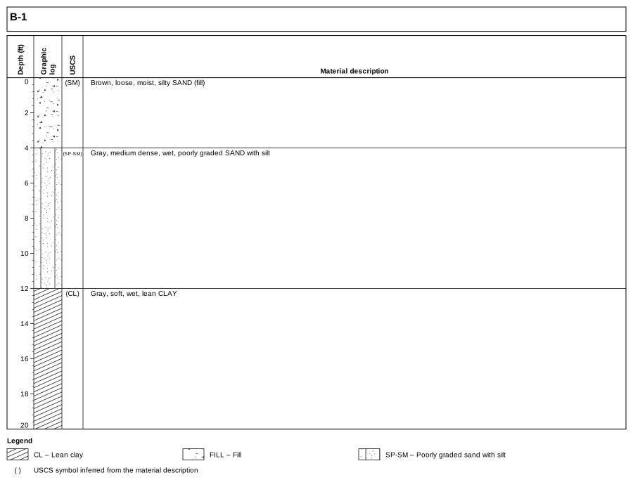
step1-layers.json. Click to open full size.Notice what it worked out on its own:
- The graphic log symbols come from the descriptions. "poorly graded SAND with silt" is drawn as SP-SM and "lean CLAY" as CL, using the ASTM D2487 group names.
- The first layer is drawn as fill, because its description ends with "(fill)".
- The USCS column shows the symbols it inferred in parentheses, so a reader can tell they weren't recorded by the logger. The legend explains the parentheses.
A symbol is inferred only when it is clear from the description. For example, "SAND" by itself doesn't give the gradation or fines information needed to classify it, so no USCS symbol is assigned. A range such as "lean to fat CLAY" similarly gets no symbol. Layers without a symbol are left blank in the graphic log. (A bare "SILT" is taken as ML.)
If you'd rather choose the symbols yourself, add a uscs field to a layer, such as "uscs": "SM". A symbol you give is shown without parentheses. It is also used for the graphic log, with two exceptions: a material named in the description (such as "(fill)") is drawn instead, and if your symbol disagrees with the description, the inferred symbol is shown below it in parentheses and the validator gives a warning. To choose the graphic log pattern outright, set hatch. See Graphic log and soil symbols for how the symbols are chosen.
A few JSON rules
JSON is strict about punctuation. If the log disappears and an error appears under the text box, it's usually one of these:
- Names and text go in double quotes:
"description": "Gray, soft, wet, lean CLAY". Numbers don't:"top": 4. - Items in a list, and fields in an object, are separated by commas, but there is no comma after the last one.
- Every
{needs a matching}, and every[a matching]. - Decimal numbers use a point:
12.5, not a comma12,5.
Click an error message to jump to the problem in the text box. The Format button re-indents the text neatly once it's valid.
Step 2: Samples, test results, groundwater and the header
Now replace the text with the complete boring:
step2-samples.jsonDownload{
"schema_version": "1.0",
"units": { "length": "ft", "unit_weight": "pcf", "diameter": "in" },
"metadata": { "project": "Example Street Bridge", "boring_name": "B-1", "elevation": 112.5, "datum": "NAVD88", "start_date": "2026-05-04", "boring_type": "Hollow-stem auger", "diameter": 8, "hammer": "Automatic trip, 140 lb", "energy_ratio": 84, "logged_by": "J. Engineer" },
"groundwater": [
{ "depth": 7.5, "date": "2026-05-04", "note": "encountered during drilling" }
],
"layers": [
{ "top": 0, "bottom": 4, "description": "Brown, loose, moist, silty SAND (fill)", "uscs": "SM" },
{ "top": 4, "bottom": 12, "description": "Gray, medium dense, wet, poorly graded SAND with silt", "uscs": "SP-SM" },
{ "top": 12, "bottom": 20, "description": "Gray, soft, wet, lean CLAY", "uscs": "CL" }
],
"samples": [
{
"top": 2.5,
"bottom": 4,
"name": "S-1",
"type": "SPT",
"blows": [3, 4, 4],
"blow_count": 8,
"specimens": [
{ "name": "S-1a", "top": 2.5, "bottom": 4, "water_content": 14.2, "fines_content": 31 }
]
},
{
"top": 7.5,
"bottom": 9,
"name": "S-2",
"type": "SPT",
"blows": [6, 9, 11],
"blow_count": 20,
"specimens": [
{ "name": "S-2a", "top": 7.5, "bottom": 9, "water_content": 22.8, "fines_content": 8 }
]
},
{
"top": 12.5,
"bottom": 14.5,
"name": "T-3",
"type": "Shelby",
"specimens": [
{ "name": "T-3a", "top": 12.6, "bottom": 13.1, "water_content": 36.5, "liquid_limit": 44, "plastic_limit": 21 },
{ "name": "T-3b", "top": 13.6, "bottom": 14.1, "water_content": 35.2, "dry_unit_weight": 84.2, "total_unit_weight": 114.9 }
],
"recovery_percent": 90
},
{
"top": 17.5,
"bottom": 19,
"name": "S-4",
"type": "SPT",
"blows": [2, 2, 3],
"blow_count": 5,
"specimens": [
{ "name": "S-4a", "top": 17.5, "bottom": 19, "water_content": 38.1 }
]
}
]
}What's new:
unitsnow also sets unit weights in pcf and diameters in inches.metadatafills the header: project, ground elevation (which adds an elevation scale), date, drilling method, borehole diameter, hammer and who logged it.groundwateris a list of water level readings, drawn as ▽ in the water level column. Every reading gets its own ▽; its date and note are listed in the legend, not beside the symbol, so they don't appear if the legend is turned off.uscson each layer gives the recorded symbol.samplesis the list of samples. Each has atopandbottomdepth, aname, a samplertype(which picks the symbol), and its blow counts. The Shelby tube also has arecovery_percent: the recovered length as a percent of the length pushed.specimens, inside each sample, are the pieces tested in the laboratory, each with its own depths and results:water_content(%),fines_content(%), unit weights,liquid_limitandplastic_limit. The Shelby tube T-3 has two.
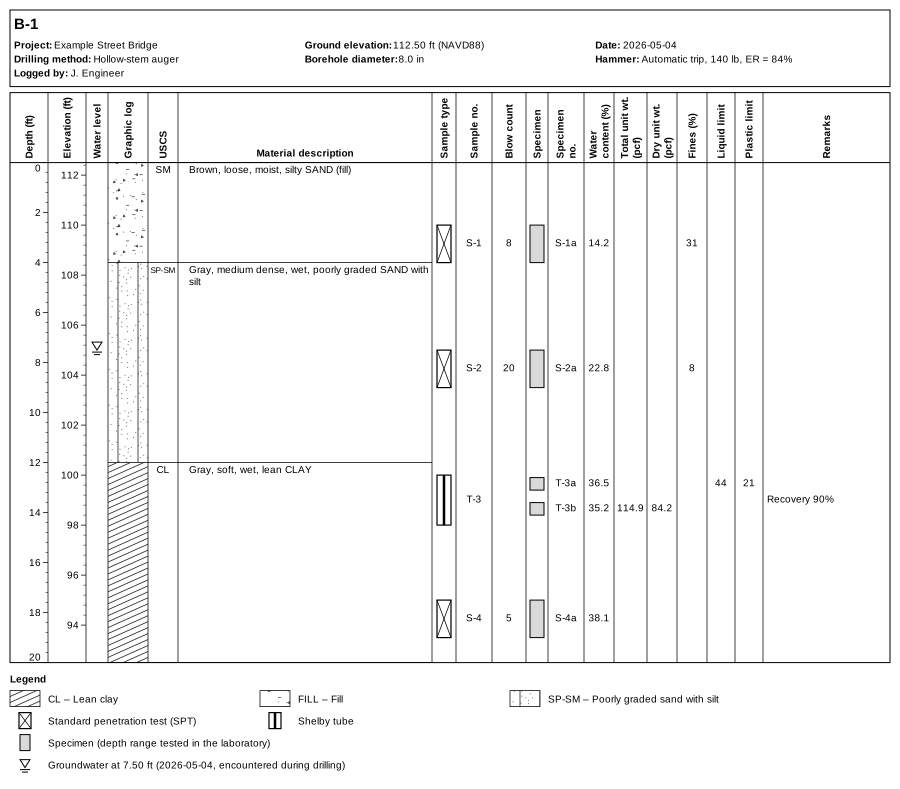
step2-samples.json. Click to open full size.Each sample's values are lined up with its sampler symbol, and each specimen's results with its grey box in the Specimen column; the depth scale stretches if needed to keep them from overlapping. The recovery is noted in the remarks. Every field is described in the data format reference; samples and specimens are explained in Samples, specimens and tests.
You only enter the data you have. The smallest log is one layer with a top and bottom. Everything else (descriptions, samples, lab results, groundwater, header fields) can be left out. When you do add an entry, a few of its fields are needed: a sample needs top and bottom, a groundwater reading needs depth, and a reference needs text. The data format reference marks these as required.
The columns follow the data: if no specimen in the log has a fines content, for example, the Fines column isn't drawn. For a single missing value, leave the field out or write null ("water_content": null). Both mean "not given", which is handy when exporting from a spreadsheet or database.
Step 3: Download or print
Above the drawing are the controls:
- Units converts the whole log to metric or US units for display, whatever units the data is in.
- Width sets the width of the drawing in pixels. Wider gives more room for descriptions.
- Header, Legend, References, Fit text and Hide empty columns turn parts of the drawing on and off. See Display options.
- Layout… (above the text box) chooses the columns, their order, widths and headings, and adds your own. See Columns and layout.
- SVG downloads a vector image: sharp at any size, editable in Inkscape or Illustrator, and best for reports.
- PNG downloads a picture at 1×, 2×, 3× or 4× (2× by default) resolution, for slides or documents that don't take SVG.
- Print / PDF opens the print dialog with only the log on the page. Choose "Save as PDF" as the printer to get a PDF.
Next steps
- Reading the log explains every part of the drawing.
- Data format reference lists every field you can use.
- Have data in Excel? Copy it into the Excel template and open the workbook in the viewer.
- Have an AGS4 or DIGGS file? Open it directly.
- Have several borings from one site? Open them all in tabs (Several logs and the map).